How To Highlight Cells In Excel Based On Text

How To Highlight Cells In Excel Based On Text – is the article you’re searching for. Hopefully, you can find information related to How To Highlight Cells In Excel Based On Text here, all of which we’ve summarized from various reliable sources.

How to Highlight Cells in Excel Based on Text

Have you ever found yourself scrolling through a spreadsheet, desperately trying to locate specific data that meets certain criteria? If so, you’re going to love this game-changing technique: highlighting cells based on text in Excel. It’s like having a built-in searchlight for your spreadsheets, instantly illuminating the information you need.

Imagine you’re working with a colossal spreadsheet containing customer data, and you want to quickly identify all customers from a particular city. With this technique, you can easily pinpoint those cells with just a few clicks. Say goodbye to endless manual searches and hello to lightning-fast data extraction.

Conditional Formatting: Your Text-Highlighting Superpower

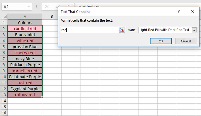
The secret lies in Excel’s Conditional Formatting feature, a powerful tool that allows you to apply formatting rules to cells based on their contents. To highlight cells based on specific text, follow these simple steps:

1. Select the range of cells you want to search.
2. Navigate to the “Home” tab in the Excel ribbon.
3. Click on “Conditional Formatting” and select “New Rule” from the drop-down menu.
4. In the “New Formatting Rule” dialog box, choose the “Use a formula to determine which cells to format” option.
5. Enter the following formula in the “Format values where this formula is true” field: =ISNUMBER(SEARCH(“text you want to find”, A2))
6. Replace “text you want to find” with the actual text you want to highlight.
7. Replace “A2” with the first cell in the range you selected in step 1.
8. Click on the “Format” button and choose a highlight color.
9. Click “OK” to apply the rule.

Example: Find & Highlight Customers from a Specific City

Let’s put this newfound knowledge into practice. Suppose you have a customer list in Excel, and you want to highlight all customers from “New York City.”

1. Select the entire customer list.
2. Follow the steps outlined in the “Conditional Formatting” section.
3. In the formula field, enter: =ISNUMBER(SEARCH(“New York City”, A2))
4. Choose a highlight color and click “OK”.

Voila! All cells containing customers from “New York City” will now be highlighted, making them easy to spot. You can leverage this technique to find and highlight any type of data in your spreadsheets, whether it’s customer names, product categories, or numeric values.

Tips & Expert Advice

• Use specific search terms: To ensure precise results, use specific and unique search terms in your formula. Avoid using common words that may appear in other cells.
• Combine multiple criteria: You can combine multiple criteria in your formula to further refine your search. For example, you can highlight cells that contain a specific text and are also within a certain date range.
• Use wildcards: Wildcards (*) can be useful when searching for partial matches. For instance, to highlight cells containing “New” or “New York,” you can use the formula: =ISNUMBER(SEARCH(“New*”, A2))
• Preview your results: Before applying the formatting, preview the results by clicking on the “Apply to” button. This allows you to double-check that the cells you want to highlight are being captured.

FAQ

• Q: Why am I not seeing any highlighted cells?

  A: Ensure that your formula is correct, that the search term is specific, and that the range you selected contains the data you want to highlight.

• Q: Can I remove the highlighting after applying it?

  A: Yes, to remove conditional formatting, select the cells with the formatting, click on “Conditional Formatting” in the Home tab, and choose “Clear Rules” from the drop-down menu.

• Q: Can I highlight cells based on case-sensitive text?

  A: Yes, to perform a case-sensitive search, use the EXACT function in your formula, e.g.: =EXACT(A2, “text you want to find”)

Conclusion

Highlighting cells based on text in Excel is a powerful technique that can significantly enhance your data analysis and visualization capabilities. By utilizing Conditional Formatting, you can quickly identify and focus on the specific information you need, saving you time and effort. Whether you’re working with large datasets or simply want to streamline your spreadsheet tasks, this technique is an invaluable addition to your Excel toolbox.

Are you ready to illuminate your spreadsheets with this game-changing technique? Give it a try and let us know how it simplifies your data exploration process.

Image: www.exceldemy.com

Thank you for visiting our website and taking the time to read How To Highlight Cells In Excel Based On Text. We hope you find benefits from this article.